Titanic Survival Prediction Machine Learning Research
Used the Kaggle Titanic dataset as a controlled machine-learning exploration sandbox. Discovered insights through EDA, engineered defensible features, benchmarked 8 model families, and selected Gradient Boosting for its stability-performance tradeoff.
Published August 2025
Case Brief
The Kaggle Titanic survival dataset is the "Hello World" of machine learning, but it serves as an excellent constrained sandbox to practice disciplined modeling.
This project was the research and prototyping phase of a two-part machine learning workflow. Before building a production-ready pipeline, I needed to uncover the true predictive signals. The goal wasn't just to maximize a leaderboard score through brute-force complexity, but to show a clean modeling journey: auditing data, engineering defensible features, benchmarking algorithms, and ultimately selecting the most stable model structure.
The output? A finalized Gradient Boosting model and a refined set of preprocessing logic ready to be modularized.
The Constraint Sandbox
The simplicity of the Kaggle Titanic dataset makes every shortcut easy to see. The raw datasets are small:
Constraints bred creativity. For instance, Age was missing for 177 passengers, Cabin for 687, and Embarked for 2. Instead of treating these purely as "data cleaning" chores, they became modeling decisions. Cabin was too sparse to lean on without creating brittle signals. Age required imputation that didn't destroy its variance.
EDA & Analytical Decisions
My exploratory data analysis focused heavily on relationships that could generalize. The important choice was restraint—avoiding the trap of overfitting an 891-row sample.
Feature Engineering
Notebook 02_feature_engineering.ipynb transitioned raw signals into 12 concrete, modeled features. The logic was crafted so it wouldn't silently break on out-of-sample data.
These transformations dramatically improved the model input space. More importantly, they clarified exactly what custom sklearn transformers I'd need to write for the production pipeline version of this project.
Algorithm Comparison & Tuning
I started with a simple baseline: applying a simple predictor using only Sex. It yielded 0.776 accuracy. A model that cannot clearly beat that baseline isn't adding enough value.
I benched eight supervised approaches to see what algorithms best mapped the feature space:
The Final Cut: XGBoost vs. Gradient Boosting
First-pass accuracy is misleading with only 891 rows, as a single split can overstate quality. I performed 5-fold cross-validation and hyperparameter grid searches on the top two:
XGBoost showed slightly higher peak cross-validation but double the fold-to-fold variance. Gradient Boosting gave nearly the same average cross-validated accuracy (0.826) but with a much lower standard deviation (0.023), indicating more consistent, stable performance.
Final Setup
The selected model was a specifically restrained GradientBoostingClassifier:
Python
GradientBoostingClassifier( n_estimators=200, learning_rate=0.1, max_depth=3, max_features="sqrt", subsample=1.0, random_state=20250708)Final performance on the validation split yielded 0.830 Accuracy (Precision: 0.802, Recall: 0.747, F1: 0.774). The confusion matrix showed 120 true negatives and 65 true positives, with only 16 false positives—proving the model learned substantially beyond the gender baseline.
Next Steps
The research phase did exactly what it was supposed to do. It acted as an exploration sandbox to identify the exact feature transformations and model family worth keeping.
The main gap? Experiment hygiene. Re-running cells from top-to-bottom works for research, but not for software.
Instead of treating the Kaggle submission (submission.csv) as the finish line, this research became the blueprint for step two: translating the notebook workflows into a robust, object-oriented system. (Read Part 2: Titanic ML Production Pipeline)
Other Projects
View all →
My website: A portfolio built with agentic AI tools
Built this portfolio as a website with agentic AI tools, using Codex, Claude, ChatGPT, Git, and Vercel instead of a no-code website builder.
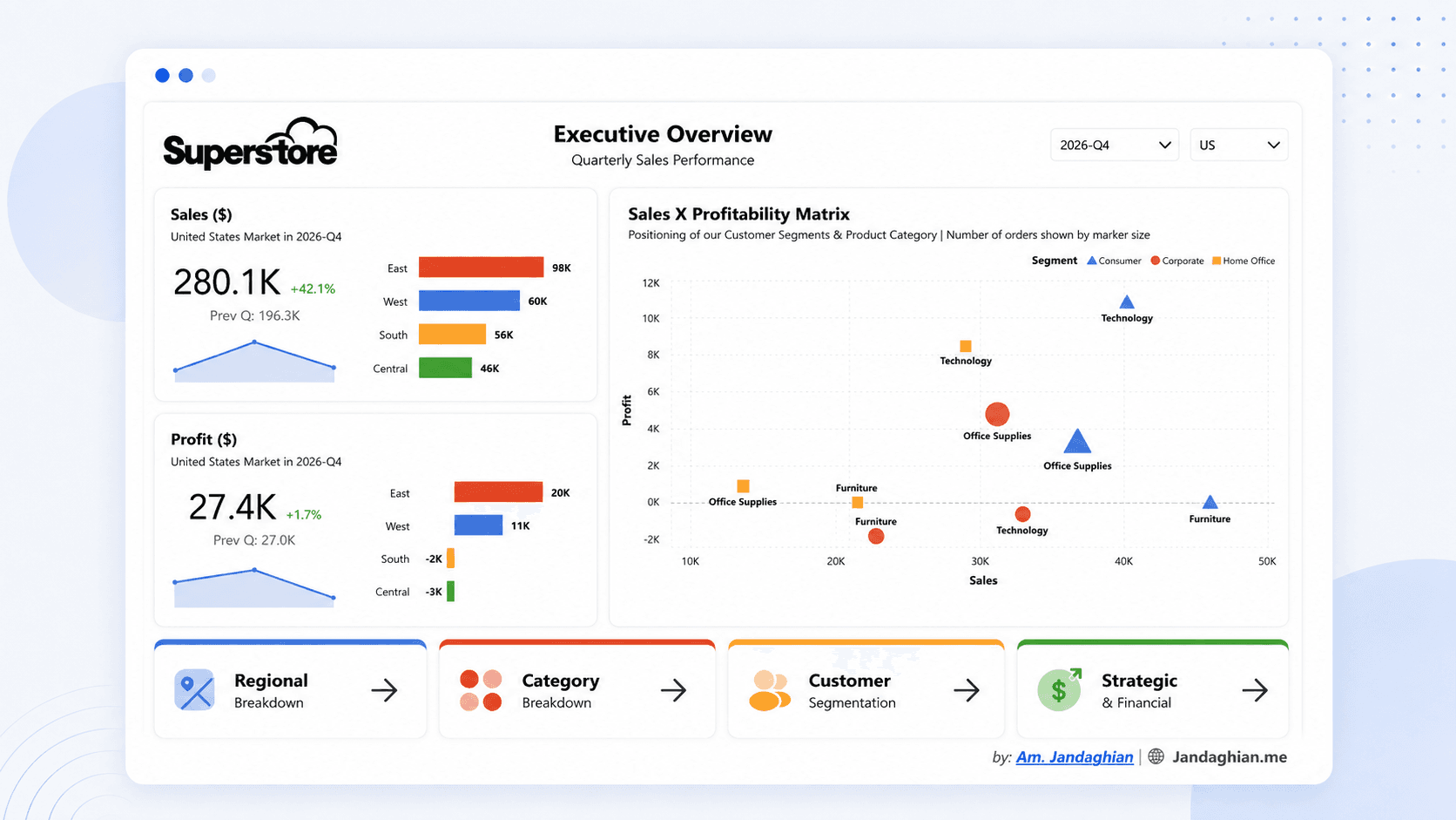
Superstore Sales Performance Dashboard
Built an executive Power BI dashboard on the Superstore dataset for quarterly sales, regional performance, categories, and customer segments.
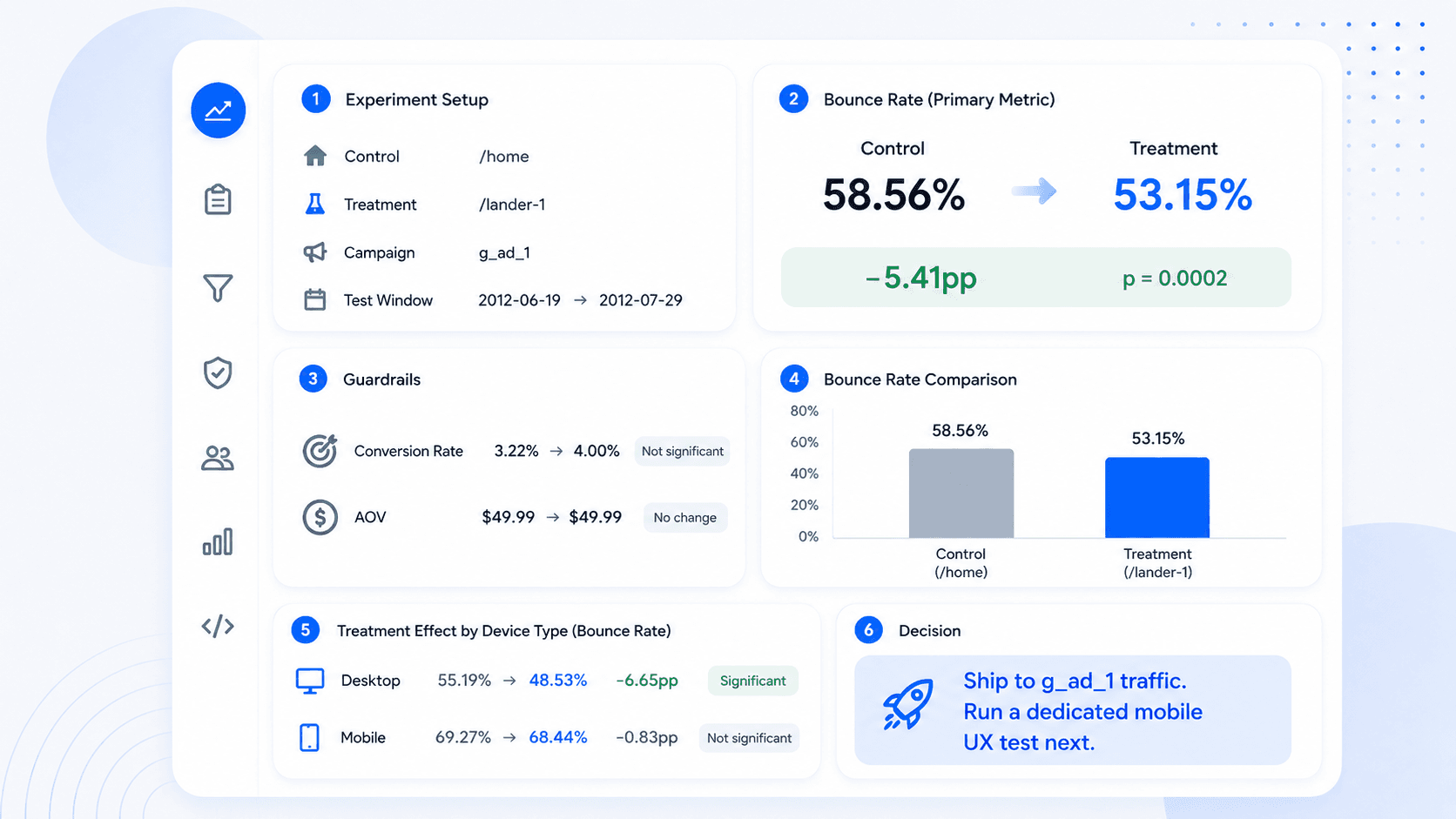
Maven Landing Page A/B Test Analysis
Analyzed a landing page experiment with traffic filtering, bounce-rate testing, guardrails, and treatment-effect cuts.
CONTACT
Want to compare notes on a project?
I'm always up for a sharp data or product conversation.
Get in touch